SWE-bench
[TOC]
1. Code Analysis
1.1 Architecture
The architecture of this benchmark can be divided into 4 layer:
- Entry Layer
- Inference Layer & Harness Layer
- Core Engine Layer
- Data Collection Layer
1 | ┌───────────────────────────────────────────────────────────────┐ |
1.2 Core Data Structure
1.2.1 SWEbenchInstance (SWE-bench Instance)
1 | class SWEbenchInstance(TypedDict): |
The core judgement of the evaluation process are
FAIL_TO_PASS and PASS_TO_PASS.
FAIL_TO_PASS: Tests that fail when the bug exists and
pass when the bug is repaired.
PASS_TO_PASS: Tests that should pass when the bug both
exists and is repaired.
1.2.2 TestSpec (Test Specification)
1 |
|
1.3.3 Three-Layer Structure of Docker Image
1 | sweb.eval.x86_64.sympy__sympy-20590:latest ← Instance Image |
Image Naming Rule :
sweb.{Layer}.{Language}.{Arch}.{Hash}:{Lable}
e.g. Test 3 different Django Issues
1 | django__django-15022 (Django 4.1, Python 3.11) |
If the docker is not layered, it is needed to create 3 different docker images:
1 | django-15022 image ──── Ubuntu + Python + Django 4.1 + Code → 2GB |
Totally 6 GB needed.
But if we layer the image:
- Base Layer: we need 2 images for Python 3.9 and Python 3.11, total 2 * 1 = 2GB.
- Env Layer: we need 2 images for Django 3.2 and Django 4.1, total 2 * 2 = 4GB
- Instance Layer: we need 3 images for each issue, total 50MB × 3 ≈ 0.15GB
- total 6.15 GB
It seems that the cost of 2 plans seem similar. But if we have 2294 instance, what will happen ?
- No layer: 2294 * 2GB = 4588 GB
- 8 images of Base Layer + 200 images of Env Layer + 2294 images of instance Layer = 8 * 1GB + 200 * 2GB + 0.15GB * 2294 ≈ 523 GB
- 88.60% Memory are saved !
1.3 Inference Pipeline
1.3.1 Default Inference (Not Available Now)
In fact, the main function of SWE-bench is to evaluate the score of patch generated by LLM. It doesn’t care about how you generate the patch. There are three original scripts to call LLM to generate patch. However there are a lot of limits of these scripts because they were just created for the paper demonstration.
There are three ways of run interference command:
Call cloud LLM API (OpenAI ChatGPT / Ahthropic Claude)
1
2
3
4python -m swebench.inference.run_api \
--dataset_name_or_path princeton-nlp/SWE-bench_oracle \
--model_name_or_path gpt-4 \
--output_dir ./outputsLocal LLM
1
2
3
4python -m swebench.inference.run_llama \
--model_name_or_path princeton-nlp/SWE-Llama-13b \
--dataset_path princeton-nlp/SWE-bench_oracle \
--output_dir ./outputsReason about issues that appear in real-time on GitHub
1
2
3python -m swebench.inference.run_live \
--model_name gpt-3.5-turbo-1106 \
--issue_url https://github.com/some/repo/issues/123
1.3.1.1 How Did The Original Inference Scripts Work?
1.3.2 How to Inference Personally
1.3.2.2 Prepare for the Env
1 | conda activate / |
1.3.2.1 Start a local LLM by vLLM (This section should be moved to Part 2 )
A local LLM has been deployed and is driven by vLLM:
1 | docker run -d --name vllm_server --gpus all \ |
1.3.2.2 Full run_local_vllm.py file
A inference script has been added:
1 | swebench/inference/run_local_vllm.py |
Parameters:
| Parameter | Type | Default | Description |
|---|---|---|---|
| –dataset_name | str | princeton-nlp/SWE-bench_Lite | Dataset: princeton-nlp/SWE-bench_Lite (300) princeton-nlp/SWE-bench_verified (500) princeton-nlp/SWE-bench (2249) |
| –split | str | test | 数据集分割:test |
| –output_dir | str | /data/disk2/wye/SWE-bench/patches_by_llm | JSONL output directory, auto-create if not exist |
| –model_short_name | str | None (Auto-Detect) | If not setted, auto-get from vLLM/v1/models |
| –max_instances | int | None(Run all instances) | Limit to only run the first N instances; 3 = test |
| –vllm_url | str | http://localhost:8000/v1 | vLLM server URL |
| –model_name | str | /models/Qwen2.5-Coder-7B-Instruct | the model’s name for vLLM |
| –max_context_files | int | 5 | context file nums for phase2 |
1.3.2.3 Inference Commnds
Start vLLM:
1 | docker run -d --name vllm_wye_swebench --gpus all \ |
Check if the vLLM is started:
1 | docker logs -f vllm_wye_swebench |
1 | cd /data/disk2/wye/SWE-bench |
Run test:
1 | python -m swebench.inference.run_local_vllm --max_instances 3 |
Run SWE-bench_Lite(default):
1 | python -m swebench.inference.run_local_vllm |
Run SWE-bench_Verified:
1 | python -m swebench.inference.run_local_vllm \ |
Run Full:
1 | python -m swebench.inference.run_local_vllm \ |
[!NOTE]
The inference script will catch the dataset automatically.
2
3
4
5
...
drwxrwxr-x 3 ubuntu ubuntu 4096 Jul 1 12:06 princeton-nlp___swe-bench_lite/
...
1.4 Evaluation Pipeline
If you run the main test command:
1 | python -m swebench.harness.run_evaluation \ |
The actual functions call chain:
1 | main() # run_evaluation.py:main() |
1.4.1 main
test split of SWE-bench Multimodal does not support the
local evaluation because of the vast cost of memory.
1 | if dataset_name == "SWE-bench/SWE-bench_Multimodal" and split == "test": |
Check ID length:
1 | assert len(run_id) > 0, "Run ID must be provided" |
Check / Create report_path:
1 | if report_dir is not None: |
SWE-bench’s docker image has 2 pulling ways (DockerHub or Local):
| namespace | Image Source | Action |
|---|---|---|
| “swebench” (default) | DockerHub | docker pull swebench/sweb.eval.xxx |
| None (pass -n none) | Local | docker build -t sweb.eval.xxx . |
force_rebuild: Only works when you use local build.
It will delete the old image and re-run docker build
command.
Load predictions (records including patches generated by
LLM for solving the issues).
And trans the list into hash map:
1 | predictions = get_predictions_from_file(predictions_path, dataset_name, split) |
Import dataset tested:
1 | dataset = get_dataset_from_preds( |
Full dataset including skipped test instances:
1 | full_dataset = load_swebench_dataset(dataset_name, split, instance_ids) |
Evaluating in the cloud:
1 | if modal: |
Evaluating locally:
Set the maximum number of file descriptors (fds) that can be opened by a process. Docker APi opens several sockets/fds for each container. The default fds num 1024 might be insufficient.
1
2
3
4if platform.system() == "Linux":
# resource.setrlimit: equal to setrlimit(2) sys call
resource.setrlimit(resource.RLIMIT_NOFILE, (open_file_limit, open_file_limit))
client = docker.from_env()recording the existing images before evaluating:
1
existing_images = list_images(client)
Dataset comes from
get_dataset_from_preds, it might be empty. The evaluation will go on only when it’s not empty. If it’s local docker image and it’s not a re-grading process, create shared dockers(base + env) for all instances:1
2
3
4
5
6
7
8
9build_env_images(
client,
dataset,
force_rebuild,
max_workers,
namespace,
instance_image_tag,
env_image_tag,
)Run all the instances(Here, each instance will generate an independent docker based on the env_images):
1
2
3
4
5
6
7
8
9
10
11
12
13
14run_instances(
predictions,
dataset,
cache_level,
clean,
force_rebuild,
max_workers,
run_id,
timeout,
namespace=namespace,
instance_image_tag=instance_image_tag,
env_image_tag=env_image_tag,
rewrite_reports=rewrite_reports,
)Clean images and generate report:
1
2
3
4
5
6
7
8
9
10clean_images(client, existing_images, cache_level, clean)
return make_run_report(
predictions,
full_dataset,
run_id,
client,
namespace,
instance_image_tag,
env_image_tag,
)
1.4.2 run_instance
1.4.2.1 whole picture
1.4.2.1.1 Preparation
入参:
1 | def run_instance( |
Initialization:
1 | instance_id = test_spec.instance_id |
rewrite_reports method (existing test_output.txt) :
1 | if rewrite_reports: |
If evaluation is interrupted mid-run, any instances whose report.json has already been written are automatically skipped on restart. This means you can safely kill the process (Ctrl+C, crash, etc.) and rerun it later — only unfinished instances will be evaluated, without duplicating completed work.
1 | if report_path.exists(): |
Create a shortcut in the logs directory, pointing to the image’s build directory. The purpose is to facilitate debugging - when you view the logs of a specific instance, you can follow this link to directly locate the corresponding Docker build files (Docker file, build logs, etc.).
1 | if not test_spec.is_remote_image: |
log:
1 | log_dir.mkdir(parents=True, exist_ok=True) |
1.4.2.1.2 Apply Patch & Run eval.sh
Env & Variable:
1 | container = None |
Prepare the eval.sh file:
1 | # eval.sh is generated dynamically by properites of TestSpec.eval_script, including: |
Run eval.sh:
1 | # record the test_output, timed_out, total_runtime |
Record the repo status( Check if the eval.sh changed the repo accidently):
1 | git_diff_output_after = ( |
1 | if git_diff_output_after != git_diff_output_before: |
1.4.2.1.3 Grading
1 | logger.info(f"Grading answer for {instance_id}...") |
1.4.2.1.4 Exception Dealing & Clear Env
Exception:
1 | except (EvaluationError, BuildImageError) as e: |
Clear Env:
1 | finally: |
1.4.2.2 eval.sh
eval.sh is generated dynamically:
1 | eval_file = Path(log_dir / "eval.sh") |
e.g:
1 |
|
1.4.2.3 get_eval_report
1 | def get_eval_report( |
Step 1 : initialize report_map
1 | report_map = {} |
now the report_map:
1 | report_map = { |
Step 2 : Check if patch exists
1 | if prediction[KEY_PREDICTION] is None: |
Step 3 : Parse test_output.txt ➡ eval_status_map
1 | eval_status_map, found = get_logs_eval(test_spec, test_log_path) |
what did get_logs_eval() do ?
1 | ① Open test_output.txt |
Step 4 : Build gold standard reference:
1 | eval_ref = { |
Step 5 : Compare item by item
1 | eval_type = EvalType.PASS_AND_FAIL |
report:
1 | report = { |
Step 6 : Final Judgement
1 | if get_resolution_status(report) == ResolvedStatus.FULL.value: |
Final Return:
1 | report_map = { |
1.4.2.4 get_resolution_status
1 | def get_resolution_status(report: dict[str, dict[str, Any]]) -> str: |
1 | def compute_fail_to_pass(report: dict[str, dict[str, Any]]) -> float: |
1.4.2.5 get_eval_tests_report
The function aims to do one thing: Classify the test cases into two categories:
FAIL_TO_PASS and PASS_TO_PASS.
Input:
1 | # real results: |
Output:
1 | { |
1.4.3 run_instances
Step 1: instance → TestSpec
1 | test_specs = list(map( |
trans JSON into TestSpec; generate all the scripts, and images’ tag;
300 instance -> 300 TestSpec.
Step 2: Check existing images
1 | existing_images = { |
Step 3: Package payloads
1 | payloads = [] |
Step 4: Thread Pool Parallelization & progress bar
1 | stats = {"✓": 0, "✖": 0, "error": 0} |
1.4.4 make_run_report
This function will traverse all instances’ report.json
1 | for instance in full_dataset: |
Clean env:
1 | if client: |
Generate Final Report:
e.g
1 | report = { |
2. Training
We can train a model to make it perform better on specific tasks like SWE-bench.
On SWE-bench, we usually use SFT + LoRA to train the model.
2.1 SFT (Supervised Fine Tuning)
The essence of SFT is that give LLM a set of [input - output] data. Then train it to imitate.
e.g. We have a 10000 pieces of data which includes:
- The Problem (issue description + relative code file)
- The Solution (repair patch)
By repeating studying those problems and solutions, the LLM will learn the ability:
1 | See similary problem -> Inference correct solution |
2.1.1 Mathematical Essence of SFT
We know that the LLM’s core thought is
Next Token Prediction. The LLM outputs token according to
the probability.
The SFT’s mathematical essence is maximizing the
conditional probability:
1 | Training Objective: |
Next Token Prediction
LLM see prompt, predict 1st token, compare the token with then one in completion -> calculate error.
LLM see prompt + 1st token, predict 2nd token, compare the token with then one in completion -> calculate error.
LLM see prompt + 1st +2nd token, predict 3rd token, compare the token with then one in completion -> calculate error.
…
LLM see prompt + 1st +2nd + … (n-1)-th token, predict n-th token, compare the token with then one in completion -> calculate error.
Total loss = average of sum of the all errors.
In fact, the error is something to evaluation the gap between the
real-token and predict-token whose real name is
Cross-Entropy.
2.1.2 Cross Entropy
2.1.2.1 Introduction
Each time the LLM predicts the next token, it will give each token in vocabulary a probability.
e.g. At one moment, the LLM’s input:
1 | "<issue>fix devide zero bug in foo.py</issue>\n<code>\ndef div(a,b):\n return |
The LLM will predict the next token, and give the candidates a probability:
1 | " def" → 0.72 |
This is the probability. But how do we
evaluate the
quality of the prediction ?
We use the Cross Entropy:
$$ \boxed{\ell = -\ln P\bigl(x_t \;\big|\; x_{<t}\bigr)} $$
- x < t = all context before position − t
- xt =
real token of position − t(comes
from the
real answerof completion ) - P(xt ∣ x < t) = LLM’s Prediction Probability to position − t with context
- ℓ = this step’s cross entropy
This formula’s essence is a Penalty Mechanism. It will
give high probability a low penalty(loss), give low probability a high
penalty (loss).
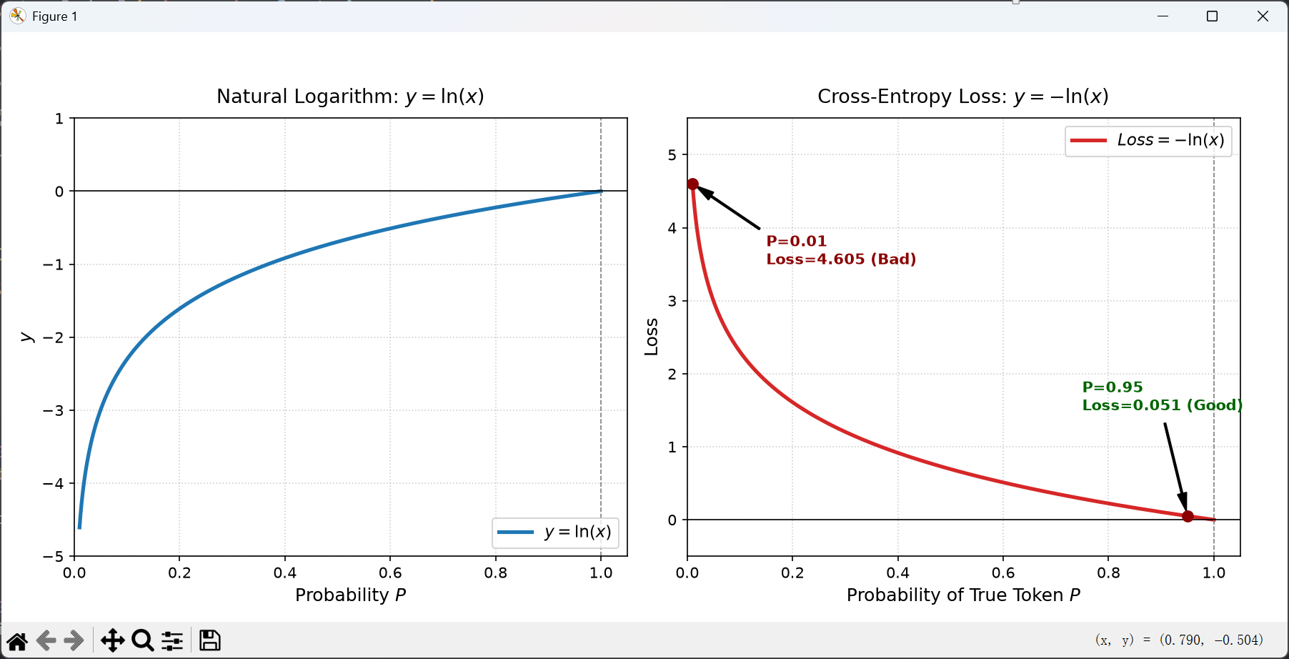
The probability P(xt | x < t) is between 0 and 1. So ln P(xt | x < t) is between −∞ and 0. So we can take the negative to have a positive interval: −ln P(xt | x < t).
How do the cross entropy work?
Example 1:
- P = 0.95
- ln (0.95) ≈ −0.051
- ℓ = 0.051
- In Optimizer’s view, the loss is very low, the prediction is very perfect. The weights is nearly needed to adjust.
Example 2:
- P = 0.01
- ln (0.01) ≈ −4.605
- ℓ = 4.605
- Optimizer will notice that
4.605is a pretty huge penalty, the weights should be adjusted substantially.
2.1.2.2 Why Use the Cross Entropy?
Why we use −ln as loss instead of using simply 1 − P?
The core thought of Cross Entropy is to Penalty the low probability. So we hope the penalty(Loss) of the low probability is extremely high. From math’s perspective, Function ln has many properties:
Loss = −ln (P)
$\frac{d\ell}{dp} = - \frac{1}{P}$
The ln ’s slope will tend towards infinity when P → 0+.
This means that if the model is very confident in a wrong prediction (for example, P=0.0001), the loss will instantly soar above 9.29.2, and the gradient of backpropagation will also be extremely large, thereby forcing the model to quickly correct those “outrageous” errors.
2.1.3 Workflow of Processing One Piece of SFT Data
SFT’s training data is assembled by
Prompt + Completion.
Assume we have one piece of data:
Prompt: "Q: Hello"
Completion: "A: Hi"; Assume
their token id:
"Q"= 10,":"= 11,"Hello"= 12"A"= 20,":"= 21,"Hi"= 22<EOS>= 50
2.1.3.1 Step 1: Concatenation & Tokenization (Build Input)
1 | tokens: [Q, :, Hello, A, :, Hi, <EOS>] |
2.1.3.2 Step 2: Build Labels
Label in machine learning area means the
Standard Answer.
LLM is a Next-Token-Prediction model. At post predict the post + 1 token.
Here the labels come from original token_ids we build:
1 | token_ids: [10, 11, 12, 20, 21, 22, 50 ] |
At index 6, no more token need to be predicted, so use
-100 as label.
2.1.3.3 Step 3: Loss Masking
The loss we discussed earlier, is a criterion to evaluate the gap
between the predicted token and
standard answer.
In SFT, we train the LLM to enhance the ability to predict the
standard answer ( The Completion).
The full input text to LLM is Prompt + Completion, we
should take the loss of Completion into consideration. So
the ability to predict the Completion will improve.
[!WARNING]
However, we should
nottake the loss of original “Prompt” into consideration. We just want LLM learn how to predict the “Completion” part instead of “Prompt” part.If LLM take the loss of
Promptinto consideration, it will repeat thePromptvery well.
So we should remove the effect of Prompt's Loss. Modify
the labels:
1 | tokens: [Q, :, Hello, A, :, Hi, <EOS>] |
We mask the labels of prediction to “Prompt”,
e.g. label(0), and label(1).
[!NOTE]
Notice that the label(2), is to predict the first token of “
Completion, do not mask it.”
2.1.3.4 Step 4: Forward Propagation & Loss Computing
Input of LLM:
1 | ["Q", ":", "Hello", "A", ":", "Hi", "<EOS>"] |
After calculating by transformer, the transformer output 7 predictions, each prediction is a set of candidates’ probability:
| Position | Context | Probability Distribution (Top 3) |
|---|---|---|
| 0 | ["Q"] |
":" → 0.85"Q" → 0.05"A" → 0.02 |
| 1 | ["Q", ":"] |
"Hello" → 0.70"Hi" →
0.15"How" → 0.05 |
| 2 | ["Q", ":", "Hello"] |
"A" → 0.60"How" →
0.10"Hi" → 0.08 |
| 3 | ["Q", ":", "Hello", "A"] |
":" → 0.90" " →
0.04"nswer" → 0.02 |
| 4 | ["Q", ":", "Hello", "A", ":"] |
"Hi" → 0.80"Hello" →
0.10"Hey" → 0.05 |
| 5 | ["Q", ":", "Hello", "A", ":", "Hi"] |
"<EOS>" →
0.95"!" → 0.02"there" →
0.01 |
| 6 | ["...", "<EOS>"] |
"The" → 0.10"A" → 0.05… |
Now we have the answer of LLM, we should grade homework by
calculating Cross Entropy according the
Masked Labels.
| Position | Label | Action | Calculation | Loss |
|---|---|---|---|---|
| 0 | -100 |
Skip | — | 0 |
| 1 | -100 |
Skip | — | 0 |
| 2 | "A" |
P → 0.60 | −log(0.60) | 0.511 |
| 3 | ":" |
P → 0.90 | −log(0.90) | 0.105 |
| 4 | "Hi" |
P → 0.80 | −log(0.80) | 0.223 |
| 5 | "<EOS>" |
P → 0.95 | −log(0.95) | 0.051 |
| 6 | -100 |
Skip | — | 0 |
All loss:
1 | [0, 0, 0.511, 0.105, 0.223, 0.051, 0] |
Mean Reduction:
We should sum the loss and get an average loss to represent the loss
of the whole answer. Notice that we should not take items of
ignore_index=-100 into the calculation.
$$ \begin{align} \mathcal{L}_{total} &= \text{MeanReduction}(\mathcal{L}_{elementwise}) \\ &= \frac{\sum_{i \in \text{Valid}} \mathcal{L}_i}{N_{\text{valid}}} \\ &= \frac{0 + 0 + 0.511 + 0.105 + 0.223 + 0.051 + 0}{4} \\ &= 0.2225 \end{align} $$
2.1.3.4 Appendix: Gradient
In a neural network, Loss Function has many independent variables.
L = f(w1, w2, ...wn)
Gradient is a column vector includes all partial derivatives all L:
$$ \begin{equation} \nabla L = \begin{bmatrix} \frac{\partial L}{\partial w_1} \\ \frac{\partial L}{\partial w_2} \\ \vdots \\ \frac{\partial L}{\partial w_n} \end{bmatrix} \end{equation} $$
Directional Derivative :
Partial Derivative like $\frac{\partial L}{\partial w_1}$, means the rate of change of L along variable w1.
Directional Derivative : rate of change of the function L along any specified direction in space.
Assume that we want to calculate the function:
L(w1, w2, ...wn)’s Directional Derivative
along unit direction vector u at point P, denoted as Du⃗L .
Core Theorem: Directional Derivative is
equal to the dot product Gradient Vector and Unit Direction
Vector(Length == 1).
Du⃗L = ∇L ⋅ u⃗
Direction of the gradient is “Direction that makes L grow fastest”.
Negative Direction
…. to be continued
2.1.3.5 Step 5: Backward Propagation & Parameters Update
Now we have the loss of this ground of generation. We should adjust our weights according to reduce the Loss.
Clear the gradient
The default design of PyTorch is gradient accumulation. If not manually reset to zero, the newly calculated gradients will be accumulated on top of the old ones, leading to a “schizophrenic” model and completely chaotic parameter updates.
1
optimizer.zero_grad()
Backward Propagation
We want to reduce the value of Loss, so we should calculate its gradient and calculate its direction.
Because of the setting-zero to the Loss of Prompt part, the
gradient component of the parameter directly related to the prediction
is also strictly 0.
Although the model “sees” the Prompt during forward
propagation, the input from the Prompt part does not make
any direct gradient contribution to the update of model parameters
during Backward propagation.
Update Weights
After calculating the gradient, the
Optimizerwill update weights according to the gradient.1
optimizer.step()
θt = θt − 1 − η ⋅ ∇θℒ(θt − 1)
AdamW:
$$ \begin{align} % 1. 计算一阶矩估计(动量 Momentum) m_t &= \beta_1 m_{t-1} + (1 - \beta_1) g_t \\ % 2. 计算二阶矩估计(未中心化的方差) v_t &= \beta_2 v_{t-1} + (1 - \beta_2) g_t^2 \\ % 3. 偏差修正(Bias Correction),防止初始阶段估计偏小 \hat{m}_t &= \frac{m_t}{1 - \beta_1^t} \\ \hat{v}_t &= \frac{v_t}{1 - \beta_2^t} \\ % 4. 最终参数更新(包含自适应步长和权重衰减) \theta_t &= \theta_{t-1} - \eta \left( \frac{\hat{m}_t}{\sqrt{\hat{v}_t} + \epsilon} + \lambda \theta_{t-1} \right) \end{align} $$