Notes on Machine Learning & Deep Learning & Reinforcement Learning
0. Reference & Notice
0.1 References
Learning Path Reference: Machine Learning Path
Main Story (Parallelism)
Stanford CS229 (Andrew Ng)
[!NOTE]
- Download / Save the notes of this course, read repeatedly.
- Solve the “Problem Sets”.
Dive into Deep Learning
Dive into Deep Learning — Dive into Deep Learning 1.0.3 documentation
Combination:
When learn some knowledge points in CS229, find them in the d2l, and implement in PyTorch.
Reference Books:
- Machine Learning, ISBN 9787302423287 (西瓜书)
- Deep Learning : Adaptive Computation and Machine Learning series, ISBN 9780262035613 (花书)
0.2 Repository
Local Repository:
1 | /e/Computer Science System Building/Deep Learning |
1. Machine Learning
2. Deep Learning
2.1 Preparation
It is planned to study with Dive into Deep Learning.
Dive into Deep Learning — Dive into Deep Learning 1.0.3 documentation
2.1.1 Install MiniConda
2.1.1.1 Install for Windows
I choose to install manually, so I download the graphical installer:
Check the 1st, 3rd item:
2.1.1.2 Configuration for GitBash
1 | /d/softwares/MiniConda/Scripts/conda init |
After initiation, the terminal displays:
1 | ==> For changes to take effect, close and re-open your current shell. <== |
However, when I restart the GitBash, the bash can’t find the command
conda, while the PowerShell can find it:
GitBash:
1
2
3test@□□ѩ□□□□ MINGW64 /e/Computer Science System Building
$ conda
bash: conda: command not foundPowerShell:
1
2(base) PS E:\Computer Science System Building> conda --version
conda 26.5.3
This because the conda init for windows writes some
configuration for PowerShell only.
So we need to write the configuration manually:
1 | echo ' |
Then restart the GitBash:
1 | test@□□ѩ□□□□ MINGW64 /e/Computer Science System Building |
2.1.2.3 Initialize a New Env
Accept new terms:
1 | conda tos accept --override-channels --channel https://repo.anaconda.com/pkgs/main |
Create new env:
1 | conda create --name d2l python=3.9 -y |
Switch to new env:
1 | conda activate d2l |
2.1.2 Install a Deep Learning Framework
Determine to install PyTorch with CUDA version 12.6 (remember to switch the env to d2l) :
1 | python -m pip install torch torchvision --index-url https://download.pytorch.org/whl/cu126 |
Check:
1 | $ python -c "import torch; print(torch.cuda.is_available()); print(torch.cuda.get_device_name(0))" |
2.1.2.1 Ideal Installation of d2l package
Install d2l package:
1 | python -m pip install d2l |
If there’s an error when you install d2l due to the high version of python (like python 13.x):
1 | $ python -m pip install d2l |
2.1.2.2 Actual Installation
I run those commands to avoid:
1 | python -m pip install d2l --no-deps |
there are some warnings that can be ignored:
1 | Installing collected packages: webencodings, pure-eval, fastjsonschema, widgetsnbextension, websocket-client, webcolors, wcwidth, urllib3, uri-template, tzdata, traitlets, tornado, tinycss2, soupsieve, six, send2trash, rpds-py, rfc3986-validator, pyzmq, pyyaml, pywinpty, python-json-logger, pyparsing, pygments, pycparser, psutil, prometheus-client, platformdirs, parso, pandocfilters, nest-asyncio2, mistune, lark, kiwisolver, jupyterlab_widgets, jupyterlab-pygments, jsonpointer, json5, idna, h11, fqdn, fonttools, executing, defusedxml, decorator, debugpy, cycler, contourpy, comm, colorama, charset_normalizer, certifi, bleach, babel, attrs, async-lru, asttokens, terminado, stack_data, rfc3987-syntax, rfc3339-validator, requests, referencing, python-dateutil, prompt_toolkit, matplotlib-inline, jupyter-core, jedi, ipython-pygments-lexers, httpcore, cffi, beautifulsoup4, anyio, pandas, matplotlib, jupyter-server-terminals, jupyter-client, jupyter-builder, jsonschema-specifications, ipython, httpx, arrow, argon2-cffi-bindings, jsonschema, isoduration, ipywidgets, ipykernel, argon2-cffi, nbformat, jupyter-console, nbclient, jupyter-events, nbconvert, jupyter-server, notebook-shim, jupyterlab-server, jupyter-lsp, jupyterlab, notebook, jupyter |
2.1.3 Open the Notebook
1
2
3mkdir d2l-en && cd d2l-en
curl https://d2l.ai/d2l-en-1.0.3.zip -o d2l-en.zip
unzip d2l-en.zip && rm d2l-en.zipEach time you should activate the env and run :
1
2
3conda activate d2l
cd pytorch
jupyter notebookThen, a progress will start on your port: http://localhost:8888 You can an run the code for each section of the book.
Whenever you open a new command line window, you will need to execute
conda activate d2lto activate the runtime environment before running the D2L notebooks, or updating your packages (either the deep learning framework or thed2lpackage). To exit the environment, runconda deactivate.
2.1.4 Notational Conventions
Numerical Objects
- x: a scalar
- x: a vector
- X: a matrix
- X: a general tensor
- I: the identity matrix (of some given dimension), i.e., a square matrix with 1 on all diagonal entries and 0 on all off-diagonals
- xi, [x]i: the ith element of vector x
- xij, xi, j, [X]ij, [X]i, j: the element of matrix X at row i and column j.
Set Theory
- 𝒳: a set
- ℤ: the set of integers
- ℤ+: the set of positive integers
- ℝ: the set of real numbers
- ℝn: the set of n-dimensional vectors of real numbers
- ℝa × b: The set of matrices of real numbers with a rows and b columns
- |𝒳|: cardinality (number of elements) of set 𝒳
- 𝒜 ∪ ℬ: union of sets 𝒜 and ℬ
- 𝒜 ∩ ℬ: intersection of sets 𝒜 and ℬ
- 𝒜 \ ℬ: set subtraction of ℬ from 𝒜 (contains only those elements of 𝒜 that do not belong to ℬ)
Functions and Operators - f(⋅): a function - log (⋅): the natural logarithm (base e) - log2(⋅): logarithm to base 2 - exp (⋅): the exponential function - 1(⋅): the indicator function; evaluates to 1 if the boolean argument is true, and 0 otherwise - 1𝒳(z): the set-membership indicator function; evaluates to 1 if the element z belongs to the set 𝒳 and 0 otherwise - (⋅)⊤: transpose of a vector or a matrix - X−1: inverse of matrix X - ⊙: Hadamard (elementwise) product - [⋅, ⋅]: concatenation - ∥ ⋅ ∥p: ℓp norm - ∥⋅∥: ℓ2 norm - ⟨x, y⟩: inner (dot) product of vectors x and y - ∑: summation over a collection of elements - ∏: product over a collection of elements - $\stackrel{\text{def}}{=}$: an equality asserted as a definition of the symbol on the left-hand side
Calculus - $\frac{dy}{dx}$: derivative of y with respect to x - $\frac{\partial y}{\partial x}$: partial derivative of y with respect to x - ∇xy: gradient of y with respect to x - ∫abf(x) dx: definite integral of f from a to b with respect to x - ∫f(x) dx: indefinite integral of f with respect to x
Probability and Information Theory - X: a random variable - P: a probability distribution - X ∼ P: the random variable X follows distribution P - P(X = x): the probability assigned to the event where random variable X takes value x - P(X ∣ Y): the conditional probability distribution of X given Y - p(⋅): a probability density function (PDF) associated with distribution P - E[X]: expectation of a random variable X - X ⟂ Y: random variables X and Y are independent - X ⟂ Y ∣ Z: random variables X and Y are conditionally independent given Z - σX: standard deviation of random variable X - Var(X): variance of random variable X, equal to σX2 - Cov(X, Y): covariance of random variables X and Y - ρ(X, Y): the Pearson correlation coefficient between X and Y, equals $\frac{\text{Cov}(X,Y)}{\sigma_X \sigma_Y}$ - H(X): entropy of random variable X - DKL(P∥Q): the KL-divergence (or relative entropy) from distribution Q to distribution P
2.2 Preliminaries
To prepare for your dive into deep learning, we will need a few survival skills:
- techniques for storing and manipulating data;
- libraries for ingesting and preprocessing data from a variety of sources;
- knowledge of the basic linear algebraic operations that we apply to high-dimensional data elements;
- just enough calculus to determine which direction to adjust each parameter in order to decrease the loss function;
- the ability to automatically compute derivatives so that you can forget much of the calculus you just learned;
- some basic fluency in probability, our primary language for reasoning under uncertainty.
- some aptitude for finding answers in the official documentation when you get stuck.
2.2.1 Data Manipulation
Generally, there are two important things we need to do with data:
- acquire them
- process them once they are inside the computer
There is no point in acquiring data without some way to store it, so to start, let’s get our hands dirty with n-dimensional arrays, which we also call tensors.
If you already know the NumPy scientific computing
package, this will be a breeze. For all modern deep learning frameworks,
the tensor class (ndarray in
MXNet, Tensor in PyTorch and
TensorFlow) resembles NumPy’s ndarray,
with a few killer features added.
First, the tensor class supports automatic differentiation.
Second, it leverages GPUs to accelerate numerical computation, whereas NumPy only runs on CPUs.
These properties make neural networks both easy to code and fast to run.
2.2.1.1 Start with Tensor
A tensor represents a (possibly multidimensional) array of numerical values.
In the one-dimensional case, i.e., when only one axis is needed for the data, a tensor is called a vector. With two axes, a tensor is called a matrix.
With K > 2 axes, we drop the specialized names and just refer to the object as a
Kth − order tensor.
PyTorch provides a variety of functions for creating new tensors prepopulated with values.
For example, by invoking arange(n), we can create a
vector of evenly spaced values, starting at 0 (included)
and ending at n (not included). By default, the interval
size is 1.
Unless otherwise specified, new tensors are stored in main memory and designated for CPU-based computation.
1 | import torch |
1 | tensor([ 0., 1., 2., 3., 4., 5., 6., 7., 8., 9., 10., 11.]) |
Each of these values is called an element of the tensor. The
tensor x contains 12 elements. We can inspect the total
number of elements in a tensor via its numel method.
1 | print("nums of elements is:", x.numel()) |
1 | nums of elements is: 12 |
We can access a tensor’s shape (the length along each axis)
by inspecting its shape attribute. Because we are dealing
with a vector here, the shape contains just a single
element and is identical to the size.
1 | print("shape of x is:", x.shape) |
1 | shape of x is: torch.Size([12]) |
We can change the shape of a tensor without altering its size or
values, by invoking reshape.
For example, we can transform our vector x whose shape
is (12,) to a matrix X with shape (3, 4).
This new tensor retains all elements but reconfigures them into a
matrix. Notice that the elements of our vector are laid out one row at a
time and thus x[3] == X[0, 3] (3rd element in x equals to
x[row 0, column 3]).
1 | print ("reshape x to 3 rows and 4 columns") |
1 | x[3] = tensor(3.) |
2.2.2 Data Processing
2.2.3 Linear Algebra
2.2.4 Calculus
2.2.5 Probability and Statistics
2.2.6 Documentation
3. Reinforcement Learning
3.1 Preparation
References Books:
- 强化学习的数学原理, 西湖大学 赵世钰
Courses:
3.2 Basic Concepts
3.2.1 A Grid World Example
Consider an example as shown in Figure, where a robot moves in a grid world. The robot, called agent, can move across adjacent cells in the grid. At each time step, it can only occupy a single cell. The white cells are accessible for entry, and the orange cells are forbidden.
There is a target cell that the robot would like to reach. We will use such grid world examples throughout this book since they are intuitive for illustrating new concepts and algorithms.
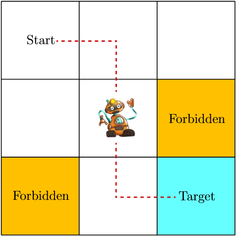
The ultimate goal of the agent is to find a “good” policy that enables it to reach the target cell when starting from any initial cell.
How can the “goodness” of a policy be defined?
- The idea is that the agent should reach the target without entering any forbidden cells, taking unnecessary detours, or colliding with the boundary of the grid.
It would be trivial to plan a path to reach the target cell if the agent knew the map of the grid world.
The task becomes nontrivial if the agent does not know any information about the environment in advance.
Then, the agent must interact with the environment to find a good policy by trial and error. To do that, the concepts presented in the rest of the chapter are necessary.
3.2.2 State & Action
State describes the Agent’s Status with respect to the environment.
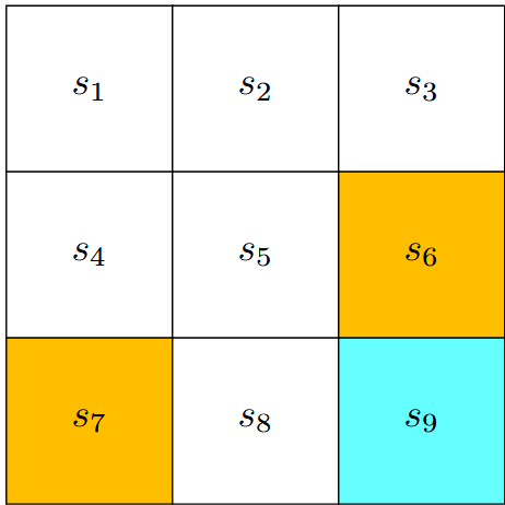
In the grid world example, the state corresponds to the agent’s location. Since there are nine cells, there are nine states as well.
They are indexed as s1, s2, ..., s9
The set of all the states is called the State Space, denoted as:
𝒮 = {s1, s2, ..., s9}
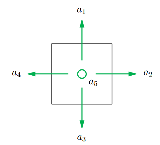
For each state, the agent can take five possible Actions:
- moving upward
- moving rightward
- moving downward
- moving leftward
- staying still
These five actions are denoted as a1, a2, ..., a5
The set of all actions is called the Action Space, denoted as:
𝒜 = {a1, a2, ..., a5}
Different states can have different action spaces.
For instance, considering that taking a1 or a4 in state s1 would lead to a collision with the boundary, we can set the action space for state s1 as:
𝒜(s1) = {a2, a3, a5}
It is considered as the most general case for all i :
𝒜(si) = {a1, ...a5}
3.2.3 State Transition
When taking an action, the agent may move from one state to another.
Such a process is called State Transition.
For example, if the agent is in state s1 and selects action a2 (that is, moving rightward), then the agent moves to state s2. Such a process can be expressed as:
$s_1 \overset{a_2}\rightarrow s_2$
2 important examples:
What’s the next state when when the agent attempts to go beyond the boundary, for example, taking action a1 in state s1?
The answer is that the agent will be bounced back because it is impossible for the agent to exit the state space. Hence, we have:
$s_1 \overset{a_1}\rightarrow s_1$
What is the next state when the agent attempts to enter a forbidden cell, for example, taking action a2 in state s5?
Two different scenarios may be encountered.
Scenario 1: Although s6 is forbidden, it is still accessible.
In this case, the next state is s6; hence, the state transition process is:
$s_5 \overset{a_2}\rightarrow s_6$
Scenario 2: s6 is not accessible because, for example, it is surrounded by walls.
In this case, the agent is bounced back to s5 if it attempts to move rightward; hence, the state transition process is:
$s_5 \overset{a_2}\rightarrow s_5$
Which scenario should we consider? The answer depends on the physical environment. In this book, we consider the first scenario where the forbidden cells are accessible, although stepping into them may get punished.
The state transition process is defined for each state and its associated actions. This process can be described by a table as shown in Table 1.1.
In this table, each row corresponds to a state, and each column corresponds to an action. Each cell indicates the next state to transition to after the agent takes an action at the corresponding state.
| a1(upward) | a2(rightward) | a3(downward) | a4(leftward) | a5(still) | |
|---|---|---|---|---|---|
| s1 | s1 | s2 | s4 | s1 | s1 |
| s2 | s2 | s3 | s5 | s1 | s2 |
| s3 | s3 | s3 | s6 | s2 | s3 |
| s4 | s1 | s5 | s7 | s4 | s4 |
| s5 | s2 | s6 | s8 | s4 | s5 |
| s6 | s3 | s6 | s9 | s5 | s6 |
| s7 | s4 | s8 | s7 | s7 | s7 |
| s8 | s5 | s9 | s8 | s7 | s8 |
| s9 | s6 | s9 | s9 | s8 | s9 |
Mathematically, the state transition process can be described by conditional probabilities.
For example, for s1 and a2, the conditional probability distribution is:
$$ \begin{aligned} p(s_1\mid s_1, a_2) = 0 \\ p(s_2\mid s_1, a_2) = 1 \\ p(s_3\mid s_1, a_2) = 0 \\ p(s_4\mid s_1, a_2) = 0 \\ p(s_5\mid s_1, a_2) = 0 \\ \end{aligned} $$
The tabular representation is only able to describe deterministic state transitions.
In general, state transitions can be stochastic and must be described by conditional probability distributions.
For instance, when random wind gusts are applied across the grid, if taking action a2 at s1, the agent may be blown to s5 instead of s2.
We have p(s5 ∣ s1, a2) > 0 in this case.
Nevertheless, we merely consider deterministic state transitions in the grid world examples for simplicity in this book.
3.2.4 Policy
A policy tells the agent which actions to take at every state.
Intuitively, policies can be depicted as arrows. Following a policy, the agent can generate a trajectory starting from an initial state.
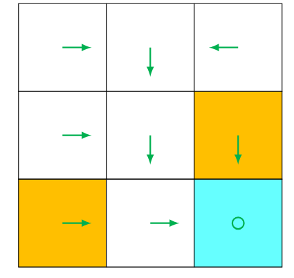
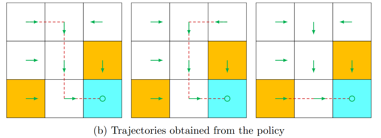
Mathematically, policies can be described by conditional probabilities.
Denote the policy as π(a ∣ s), which is a conditional probability distribution function defined for every state.
For example, the policy for s1 is:
$$ \begin{aligned} \pi (a_1\mid s_1)= 0 \\ \pi (a_2\mid s_1)= 1 \\ \pi (a_3\mid s_1)= 0 \\ \pi (a_4\mid s_1)= 0 \\ \pi (a_5\mid s_1)= 0 \\ \end{aligned} $$
The above policy is deterministic. Policies may be stochastic in general.
For example, the policy shown is stochastic: in state s1, the agent may take actions to go either rightward or downward. The probabilities of taking these two actions are the same (both are 0.5).
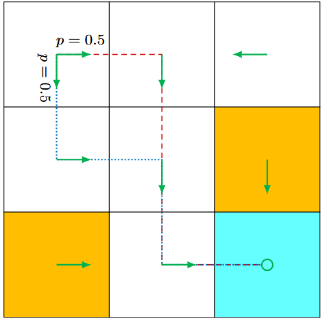
In this case, the policy for s1 is:
$$ \begin{aligned} &\pi (a_1\mid s_1)= 0 \\ &\pi (a_2\mid s_1)= 0.5 \\ &\pi (a_3\mid s_1)= 0.5 \\ &\pi (a_4\mid s_1)= 0 \\ &\pi (a_5\mid s_1)= 0 \end{aligned} $$
Policies represented by conditional probabilities can be stored as tables.
Table represents the stochastic policy depicted in the figure above.
| a1(upward) | a2(rightward) | a3(downward) | a4(leftward) | a5(still) | |
|---|---|---|---|---|---|
| s1 | 0 | 0.5 | 0.5 | 0 | 0 |
| s2 | 0 | 0 | 1 | 0 | 0 |
| s3 | 0 | 0 | 0 | 1 | 0 |
| s4 | 0 | 1 | 0 | 0 | 0 |
| s5 | 0 | 0 | 1 | 0 | 0 |
| s6 | 0 | 0 | 1 | 0 | 0 |
| s7 | 0 | 1 | 0 | 0 | 0 |
| s8 | 0 | 1 | 0 | 0 | 0 |
| s9 | 0 | 0 | 0 | 0 | 1 |
3.2.5 Reward
Reward is one of the most unique concepts in reinforcement learning.
After executing an action at a state, the agent obtains a reward, denoted as r, as feedback from the environment.
The reward is a function of the state s and action a.
Hence, it is also denoted as r(s, a).
Its value can be a positive or negative real number or zero.
Generally speaking, with a positive reward, we encourage the agent to take the corresponding action. With a negative reward, we discourage the agent from taking that action.
In the grid world example, the rewards are designed as follows:
- If the agent attempts to exit the boundary, rboundary = −1
- If the agent attempts to enter a forbidden cell, rforbidden = −1
- If the agent reaches the target state, rtarget = 1
- Otherwise, the agent obtains a reward of rother = 0
Special attention should be given to the target state s9.
The reward process does not have to terminate after the agent reaches s9.
- If the agent takes action a5 at s9, the next state is again s9, and the reward is rtarget = +1 .
- If the agent takes action a2, the next state is also s9, but the reward is rboundary = −1.
A reward can be interpreted as a human-machine interface, with which we can guide the agent to behave as we expect.
For example, with the rewards designed above, we can expect that the agent tends to avoid exiting the boundary or stepping into the forbidden cells.
Designing appropriate rewards is an important step in reinforcement learning.
The process of getting a reward after executing an action can be intuitively represented as a table, as shown in Table below. Each row of the table corresponds to a state, and each column corresponds to an action. The value in each cell of the table indicates the reward that can be obtained by taking an action at a state.
One question that beginners may ask is as follows:
- If given the table of rewards, can we find good policies by simply selecting the actions with the greatest rewards?
- The answer is no.
That is because these rewards are immediate rewards that can be obtained after taking an action. To determine a good policy, we must consider the total reward obtained in the long run.
An action with the greatest immediate reward may not lead to the greatest total reward.
Local Optimum ≠ Global Optimum
Although intuitive, the tabular representation is only able to describe deterministic reward processes. A more general approach is to use conditional probabilities p(r ∣ s, a) to describe reward processes. For example, for state s1, we have:
p(r = −1 ∣ s1, a1) = 1
p(r ≠ −1 ∣ s1, a1) = 0
| a1(upward) | a2(rightward) | a3(downward) | a4(leftward) | a5(still) | |
|---|---|---|---|---|---|
| s1 | rboundary | 0 | 0 | rboundary | 0 |
| s2 | rboundary | 0 | 0 | 0 | 0 |
| s3 | rboundary | rboundary | rforbidden | 0 | 0 |
| s4 | 0 | 0 | rforbidden | rboundary | 0 |
| s5 | 0 | rforbidden | 0 | 0 | 0 |
| s6 | 0 | rboundary | rtarget | 0 | rforbidden |
| s7 | 0 | 0 | rboundary | rboundary | rforbidden |
| s8 | 0 | rtarget | rboundary | rforbidden | 0 |
| s9 | rforbidden | rboundary | rboundary | 0 | rtarget |
In this example, the reward process is deterministic. In general, it can be stochastic. For example, if a student studies hard, he or she would receive a positive reward (e.g., higher grades on exams), but the specific value of the reward may be uncertain.
3.2.6 Trajectories, Returns and Episodes
A trajectory is a state-action-reward chain.
Trajectories obtained by following two policies. The trajectories are indicated by red dashed lines.
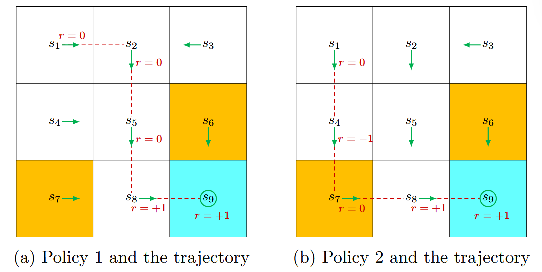
For example, given the policy shown in Figure (a), the agent can move along a trajectory as follows:
$s_1 \xrightarrow[r_0]{a_1} s_2 \xrightarrow[r_0]{a_3} s_5 \xrightarrow[r_0]{a_3} s_8 \xrightarrow[r_{target}]{a_2} s_9$
Return:
Returns are also called total rewards or cumulative rewards.
Ther return of the trajectory above is:
return = 0 + 0 + 0 + 1 = 1
Returns can be used to evaluate policies.
For example, we can evaluate the two policies in Figure by comparing their returns.
Left policy: 1
Right policy:
$s_1 \xrightarrow[r_0]{a_3} s_4 \xrightarrow[{r=-1}]{a_3} s_7 \xrightarrow[r_0]{a_2} s_8 \xrightarrow[r_{target}]{a_2} s_9$
return = 0 − 1 + 0 + 1 = 0
The returns in (1.1) and (1.2) indicate that the left policy is better than the right one since its return is greater.
A return consists of an immediate reward and future rewards. Here, the immediate reward is the reward obtained after taking an action at the initial state; the future rewards refer to the rewards obtained after leaving the initial state.
It is possible that the immediate reward is negative while the future reward is positive. Thus, which actions to take should be determined by the return (i.e., the total reward) rather than the immediate reward to avoid short-sighted decisions.
Return can also be defined for infinitely long trajectories.
For example, the trajectory in Figure stops after reaching s9. Since the policy is well defined for s9, the process does not have to stop after the agent reaches s9.
We can design a policy so that the agent stays still after reaching s9. Then, the policy would generate the following infinitely long trajectory:
$s_1 \xrightarrow[r_0]{a_1} s_2 \xrightarrow[r_0]{a_3} s_5 \xrightarrow[r_0]{a_3} s_8 \xrightarrow[r_{target}]{a_2} s_9 \xrightarrow[{r=1}]{a_5}s_9 \xrightarrow[{r=1}]{a_5}s_9...$
The direct sum of the rewards along this trajectory is:
return = 0 + 0 + 0 + 1 + 1 + 1... = ∞
Therefore, we must introduce the discounted return concept for infinitely long trajectories. In particular, the discounted return is the sum of the discounted rewards:
Discount Rate, γ:
γ ∈ (0, 1)
Discounted Return:
$$ \begin{aligned} \text{Return} =& \ 0 + 0 + 0 + 1 + 1 + 1 +... \\ \text{Discounted Return} =& \gamma^0\cdot0 + \gamma^1\cdot0 + \gamma^2\cdot0 + \gamma^3\cdot1+\gamma^4\cdot1 + \gamma^5\cdot1+...\\ =& \gamma^3(1+\gamma+\gamma^2+...)\\ =& \gamma^3\frac{1}{1-\gamma} \end{aligned} $$
By introduce Dicounted Rate, we make the return become finite.
And we can balance the far rewards and near rewards:
Discounted Return = γ0 ⋅ 0 + γ1 ⋅ 0 + γ2 ⋅ 0 + γ3 ⋅ 1 + γ4 ⋅ 1 + γ5 ⋅ 1 + ...
- γ is close to 0: the high-order terms like(γ5, γ6...) will converge rapidly.
- γ is close to 1: the high-order terms like(γ5, γ6...) will accumulate more, and the weights will increase.
In a nutshell:
By control the γ, we can determine the agent is more short-sight or long-sight
Now let’s talk about Episodes:
When interacting with the environment by following a policy, the agent may stop at some terminal states. The resulting trajectory is called an episode (or a trial ).
If the environment or policy is stochastic, we obtain different episodes when starting from the same state.
However, if everything is deterministic, we always obtain the same episode when starting from the same state.
An episode is usually assumed to be a finite trajectory. Tasks with episodes are called episodic tasks. However, some tasks may have no terminal states, meaning that the process of interacting with the environment will never end. uch tasks are called continuing tasks.
In fact, we can treat episodic and continuing tasks in a unified mathematical manner by converting episodic tasks to continuing ones. Specifically, after reaching the terminal state in an episodic task, the agent can continue taking actions in the following two ways.
If we treat the terminal state as a special state, we can specifically design its action space or state transition so that the agent stays in this state forever. Such states are called absorbing states, meaning that the agent never leaves a state once reached.
For example, for the target state s9, we can specify 𝒜(s9) = {a5} or set 𝒜(s9) = {a1, ..., a5} with p(s9|s9, ai) = 1 for all i = 1,...,5
Second, if we treat the terminal state as a normal state, we can simply set its action space to the same as the other states, and the agent may leave the state and come back again.
Since a positive reward of r = 1 can be obtained every time s9 is reached, the agent will eventually learn to stay at s9 forever to collect more rewards.
Notably, when an episode is infinitely long and the reward received for staying at s9 is positive, a discount rate must be used to calculate the discounted return to avoid divergence.
In this book, we consider the second scenario where the target state is treated as a normal state whose action space is 𝒜(s9) = {a1, ..., a5}.
3.2.7 Markov Decision Processes
Markov Decision Processes is a general framework for describing stochastic dynamical systems. The key ingredients of an MDP are listed below:
Sets:
- State Space: the set of all states, denoted as 𝒮.
- Action Space: a set of actions, denoted as 𝒜(s), associated with each state s ∈ S.
- Reward Set: a set of rewards, denoted as ℛ(s, a), associated with each state-action pair (s, a)
Model:
- State transition probability: In state s, when taking action a, the probability of transitioning to state s′ is p(s ∣ s, a). It holds that ∑s′ ∈ 𝒮p(s′ ∣ s, a) = 1 for any (s, a).
- Reward probability: In state s, when taking action a, the probability of obtaining reward r is p(r ∣ s, a). It holds that ∑r ∈ ℛp(r ∣ s, a) = 1 for any (s, a).
Markov Property: The Markov Property refers to the memoryless property of a stochastic process. Mathematically, it means that:
$$ \begin{aligned} p(s_{t+1}|s_t,a_t,s_{t-1},a_{t-1},...,s_0,a_0) = p(s_{t+1}|s_t,a_t)\\ p(r_{t+1}|s_t,a_t,s_{t-1},a_{t-1},...,s_0,a_0) = p(r_{t+1}|s_t,a_t) \end{aligned} $$
Where t represents the current time step and t + 1 represents the next time step. The next state or reward depends merely on the current state and action and is independent of the previous ones.
The Markov property is important for deriving the fundamental Bellman equation of MDPs.
Here, p(s′ ∣ s, a) and p(r ∣ s, a) for all (s, a) are called the model or dynamics
The model can be either stationary or nonstationary (or in other words, time-invariant or time-variant).
A stationary model does not change over time; a nonstationary model may vary over time. For instance, in the grid world example, if a forbidden area may pop up or disappear sometimes, the model is nonstationary. In this book, we only consider stationary models.
One may have heard about the Markov Processes (MPs). What is the difference between an MDP and an MP?
The answer is that, once the policy in an MDP is fixed, the MDP degenerates into an MP.
The agent is a decision-maker that can sense its state, maintain policies, and execute actions. Everything outside of the agent is regarded as the environment.
3.2.8 Q&A
Q: Can we set all the rewards as negative or positive?
A: In fact, it is the relative reward values instead of the absolute values that determine encouragement or discouragement. More specifically, we set:
$$ \begin{aligned} r_\text{boundary} =& -1 \\ r_\text{forbidden} =& -1 \\ r_\text{target} =& +1 \\ r_\text{other} =& 0 \end{aligned} $$
We can also add a common value to all these values without changing the resulting optimal policy. For example, we can add −2 to all the rewards to obtain:
$$ \begin{aligned} r_\text{boundary} =& -3 \\ r_\text{forbidden} =& -3 \\ r_\text{target} =& -1 \\ r_\text{other} =& -2 \end{aligned} $$
Although the rewards are all negative, the resulting optimal policy is unchanged. That is because optimal policies are invariant to affine transformations of the rewards.
Q: Is the reward a function of the next state?
A: We mentioned that the reward r depends only on s and a but not the next state s′. However, this may be counterintuitive since it is the next state that determines the reward in many cases.
For example, the reward is positive when the next state is the target state. As a result, a question that naturally follows is whether a reward should depend on the next state.
A mathematical rephrasing of this question is whether we should use p(r|s, a, s′) where s′ is the next state rather than p(r|s, a).
The answer is that r depends on s, a, and s′.
However, since s′ also depends on s and a, we can equivalently write r as a function of s and a:
p(r ∣ s, a) = ∑s′p(r ∣ s, a, s′) p(s′ ∣ s, a)
In a stochastic environment, specified s and a might induce different s′; The final reward is dependent on the previous state and action by Total Probability Theorem.
3.3 Bellman Equation
3.3.1 returns
In fact, returns play a fundamental role in reinforcement learning since they can evaluate whether a policy is good or not. This is demonstrated by the following examples.
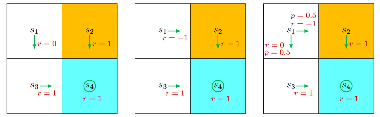
There are three policies shown above. We can use 𝓇ℯ𝓉𝓊𝓇𝓃𝓈 to evaluate the policies’ quality.
$$ \begin{align*} \text{return}_1 &= 0+\gamma\cdot 1+\gamma^2\cdot 1+\gamma^3\cdot 1+\cdots \\ &= \frac{\gamma}{1-\gamma} \\[2ex] \text{return}_2 &= -1+\gamma\cdot 1+\gamma^2\cdot 1+\gamma^3\cdot 1+\cdots \\ &= \frac{\gamma}{1-\gamma}-1 \\[2ex] \text{return}_3 &= 0.5 \left(\frac{\gamma}{1-\gamma}\right) +0.5 \left(\frac{\gamma}{1-\gamma}-1\right) \\ &= \frac{\gamma}{1-\gamma}-0.5 \end{align*} $$
So it is obviously that the qualities are:
return1 > return3 > return2
3.3.2 Calculate Returns
Here’s a state transition illustration:
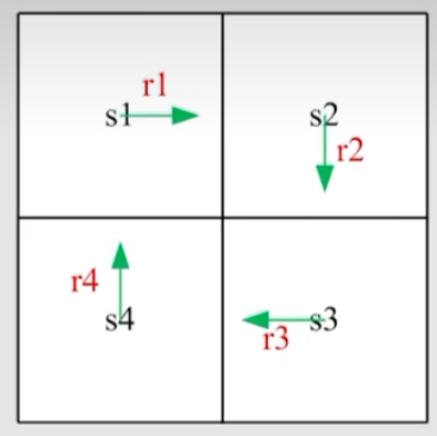
The returns from different start position can are denoted as vi:
$$ \begin{aligned} v_1 &= r_1 + \gamma \cdot r_2 + \gamma^2 \cdot r_3 + \gamma^3 \cdot r_4 + \cdots \\ v_2 &= r_2 + \gamma \cdot r_3 + \gamma^2 \cdot r_4 + \gamma^3 \cdot r_1 + \cdots \\ v_3 &= r_3 + \gamma \cdot r_4 + \gamma^2 \cdot r_1 + \gamma^3 \cdot r_2 + \cdots \\ v_4 &= r_4 + \gamma \cdot r_1 + \gamma^2 \cdot r_2 + \gamma^3 \cdot r_3 + \cdots \end{aligned} $$
Obviously, the equation can be written as:
$$ \begin{align*} v_1 &= r_1 + \gamma \cdot r_2 + \gamma ^2 \cdot r_3 + \gamma ^3 \cdot r_4 + \dots = r_1 + \gamma \left(v_2\right) \\ v_2 &= r_2 + \gamma \cdot r_3 + \gamma ^2 \cdot r_4 + \gamma ^3 \cdot r_1 + \dots = r_2 + \gamma \left(v_3\right) \\ v_3 &= r_3 + \gamma \cdot r_4 + \gamma ^2 \cdot r_1 + \gamma ^3 \cdot r_2 + \dots = r_3 + \gamma \left(v_4\right) \\ v_4 &= r_4 + \gamma \cdot r_1 + \gamma ^2 \cdot r_2 + \gamma ^3 \cdot r_3 + \dots = r_4 + \gamma \left(v_1\right) \\ \end{align*} $$
We can transform the equation into a matrix-vector format:
$$ \begin{aligned} \begin{pmatrix}v_1\\v_2\\v_3\\v_4\end{pmatrix} &= \begin{pmatrix}r_1\\r_2\\r_3\\r_4\end{pmatrix} + \gamma \begin{pmatrix}v_2\\v_3\\v_4\\v_1\end{pmatrix} \\ &= \begin{pmatrix}r_1\\r_2\\r_3\\r_4\end{pmatrix} + \gamma \begin{pmatrix} 0&1&0&0\\ 0&0&1&0\\ 0&0&0&1\\ 1&0&0&0 \end{pmatrix} \begin{pmatrix}v_1\\v_2\\v_3\\v_4\end{pmatrix} \end{aligned} $$
Denote:
$$ \Pi = \begin{pmatrix} 0&1&0&0\\ 0&0&1&0\\ 0&0&0&1\\ 1&0&0&0 \end{pmatrix} $$
Then we have:
v = r + γ Π v
This is the basic bellman equation.
Solution:
$$ \begin{aligned} \mathbf{v}&=\mathbf{r}+\gamma\,\Pi\,\mathbf{v} \\ \left(\mathbf{E}-\gamma\,\Pi\right)\,\mathbf{v} &= \mathbf{r}\\ \mathbf{v} &= \mathbf{r}\,\left(\mathbf{E}-\gamma\,\Pi\right)^{-1} \end{aligned} $$
3.3.3 State Value
Consider a single-step process:
$$ S_t \xrightarrow{A_t} R_{t+1},S_{t+1} $$
- t, t + 1: discrete time instances
- St: State at time t
- At: Action at time t
- Rt + 1: Reward obtained after taking action At
- St + 1: State transited after taking action At
Note: the St, At, Rt + 1, St + 1 are all random variables.
This step is governed by the following probability distribution:
- St → At is governed by π(At = a ∣ St = s)
- St, At → Rt + 1 is governed by p(Rt + 1 = r ∣ St = s, At = t)
- St, At → St + 1 is governed by p(St + 1 = s′ ∣ St = s, At = t)
For a multi-step trajectory:
$$ S_t \xrightarrow {A_t}R_{t+1}, S_{t+1}\xrightarrow {A_{t+1}}R_{t+2}, S_{t+2}\xrightarrow {A_{t+2}}R_{t+3}, S_{t+3} \cdots $$
The discounted return is:
Gt = Rt + 1 + γ Rt + 2 + γ2 Rt + 3…
- γ ∈ (0, 1) is a discount rate.
- Gt is also a random variable since Rt + 1, Rt + 2 are random variables.
The expectation ( or called expected value or mean ) of Gt is defined as the state-value function or simply state value:
vπ(s) = 𝔼[Gt ∣ St = s]
- It is a function of s. It is a conditional expectation with the condition that the state starts from s.
- It is based on policy π. The vπ(s) also can be written as v(π, s).
Q: What is the difference between return and state value?
A: return is result of a single trajectory, while the state value is a expectation of many different trajectories. If everything including π(a ∣ s), p(r ∣ a, s), p(s′ ∣ a, s) us deterministic, the state value is the same as the return.
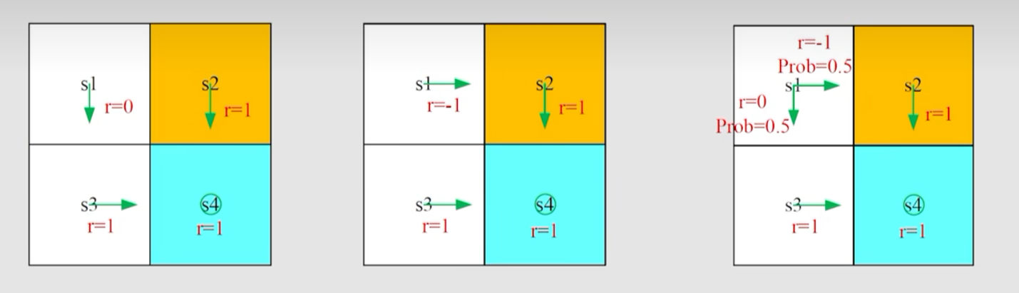
The three pictures have corresponding policies π1, π2, and π3.
The corresponding state values are:
$$ \begin{aligned} v_{\pi}(s_1) &= 0 + \gamma\cdot1+\gamma^2\cdot1\dots = \gamma\left(1+1^2+\dots\right) = \gamma\,\frac{1-\gamma^n}{1-\gamma} = \frac{\gamma}{1-\gamma} \\ v_{\pi}(s_2) &= -1 + \gamma\cdot1+\gamma^2\cdot1\dots = -1 +\gamma\,\frac{1-\gamma^n}{1-\gamma} = \frac{\gamma}{1-\gamma}-1 \\ v_{\pi}(s_3) &= 0.5 \times\frac{\gamma}{1-\gamma}+0.5 \times \left(\frac{\gamma}{1-\gamma}-1\right) = \frac{\gamma}{1-\gamma}-0.5 \end{aligned} $$